Python language:
Briefly summarize the common features of the Python language in data analysis and mining scenarios:
List (can be modified), tuple (cannot be modified)
dictionary(
Collection (same set of mathematical concepts)
Functional programming (mainly composed of lambda(), map(), reduce(), filter())
Python data analysis common library:

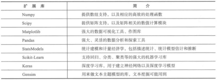
Python data mining related extension library
NumPy
Providing a real array is faster than Python's built-in list. NumPy is also a dependency library for libraries such as Scipy, Matplotlib, and Pandas. Built-in functions handle data at a C-level, so you should use built-in functions whenever possible.
Example: NumPy basic operation
Import numpy as np # is generally aliased with np a = np.array([2, 0, 1, 5]) print(a) print(a[:3]) print(a.min()) a.sort( ) # a is overprinted print(a) b = np.array([[1, 2, 3], [4, 5, 6]]) print(b*b)
Output:
[2 0 1 5] [2 0 1] 0 [0 1 2 5] [[ 1 4 9] [16 25 36]]
Scipy
NumPy and Scipy give Python a taste of MATLAB. Scipy relies on NumPy, which provides multidimensional array functionality, but just a generic array is not a matrix. For example, when two arrays are multiplied, only the corresponding elements are multiplied. Scipy provides real matrices, as well as a large number of objects and functions based on matrix operations.
Scipy contains functions such as optimization, linear algebra, integration, interpolation, fitting, special functions, fast Fourier transform, signal processing, image processing, and ordinary differential equation solving.
Example: Scipy solves nonlinear equations and numerical integration
# solved the equations from scipy.optimize import fsolve def f(x): x1 = x[0] x2 = x[1] return [2 * x1 - x2 ** 2 - 1, x1 ** 2 - x2 - 2] Result = fsolve(f, [1, 1]) print(result) # integral from scipy import integrate def g(x): # define integrand function return (1 - x ** 2) ** 0.5 pi_2, err = integrate .quad(g, -1, 1) # Output integration result and error print(pi_2 * 2, err)
Output:
[ 1.91963957 1.68501606] 3.141592653589797 1.0002356720661965e-09
Matplotlib
The famous drawing library in Python, mainly used for 2D drawing, and can also be used for simple 3D drawing.
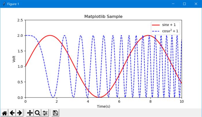
Example: Matplotlib drawing basic operations
Import matplotlib.pyplot as plt import numpy as np x = np.linspace(0, 10, 10000) # argument x, 10000 is the number of points y = np.sin(x) + 1 # dependent variable yz = np. Cos(x ** 2) + 1 # dependent variable z plt.figure(figsize=(8, 4)) # Set image size # plt.rcParams['font.sans-serif'] = 'SimHei' # In Chinese, you need to set the font # plt.rcParams['axes.unicode_minus'] = False # If the negative sign is not displayed properly when saving the image, add the sentence # two curves plt.plot(x, y, label='$ \sin (x+1)$', color='red', linewidth=2) # Set the label, line color, line size plt.plot(x, z, 'b--', label='$\cos x ^2+1$') plt.xlim(0, 10) # x coordinate range plt.ylim(0, 2.5) # y coordinate range plt.xlabel("Time(s)") # x axis name plt.ylabel( "Volt") # y-axis name plt.title("Matplotlib Sample") #å›¾çš„æ ‡é¢˜plt.legend() # Show legend plt.show() # Show drawing results
Output:

Pandas
Pandas is a very powerful data analysis tool in Python. It is built on top of NumPy, it is very powerful, supports SQL-like additions and deletions, and has rich data processing functions, supports time series analysis, and supports flexible processing of missing data.
The basic data structures of Pandas are Series and DataFrame. Series is a sequence, similar to a one-dimensional array, DataFrame is equivalent to a two-dimensional table, similar to a two-dimensional array, each column is a Series. To locate the elements in the Series, Pandas provides an Index object, similar to the primary key.
DataFrame is essentially a container for Series.
Example: Pandas simple operation
Import pandas as pd s = pd.Series([1, 2, 3], index=['a', 'b', 'c']) d = pd.DataFrame([[1, 2, 3], [ 4, 5, 6], [7, 8, 9], [10, 11, 12], [13, 14, 15], [16, 17, 18]], columns=['a', 'b' , 'c']) d2 = pd.DataFrame(s) print(s) print(d.head()) # Preview the first 5 lines print(d.describe()) # Read the file (the path is best not to have Chinese ) df=pd.read_csv("G:\\data.csv", encoding="utf-8") print(df)
Output:
a 1 b 2 c 3 dtype: int64 abc 0 1 2 3 1 4 5 6 2 7 8 9 3 10 11 12 4 13 14 15 abc count 6.000000 6.000000 6.000000 mean 8.500000 9.500000 10.500000 std 5.612486 5.612486 5.612486 min 1.000000 2.000000 3.000000 25% 4.750000 5.750000 6.750000 50% 8.500000 9.500000 10.500000 75% 12.250000 13.250000 14.250000 max 16.000000 17.000000 18.000000 Empty DataFrame Columns: [1068, 12, fruits and vegetables, 1201, vegetables, 120104, flowers, 20150430, 201504, DW-1201040010, scattered, fresh, Kilograms, 0.973, 5.43, 2.58, no] Index: []
Scikit-Learn
Scikit-Learn relies on NumPy, Scipy, and Matplotlib, and is a powerful machine learning library in Python that provides features such as data preprocessing, classification, regression, clustering, prediction, and model analysis.
Example: Creating a linear regression model
From sklearn.linear_model import LinearRegression model= LinearRegression() print(model)
Interfaces provided by all models:
Model.fit(): training model, the supervised model is fit(X,y), and the unsupervised model is fit(X)
The interface provided by the monitoring model:
Model.predict(X_new): predicts the new sample model.predict_proba(X_new): predictive probability, useful only for certain models (LR)
Interface provided by the unsupervised model:
Model.ransform(): Learn from the data the new "base space" model.fit_transform(): the new base learned from the data and convert this data according to this set of "bases"
Scikit-Learn itself comes with some data sets, such as flowers and handwritten image data sets. Below is a chestnut with a flower data set. The training set contains 4 dimensions - the length, width, length and width of the petals, and four Subgenus classification results.
Example:
From sklearn import datasets # Import dataset from sklearn import svm iris = datasets.load_iris() # Load dataset clf = svm.LinearSVC() # Create linear SVM classifier clf.fit(iris.data, iris.target) #用Data training model print(clf.predict([[5, 3, 1, 0.2], [5.0, 3.6, 1.3, 0.25]]))
Output:
[0 0]
Keras
Keras is based on Theano's deep learning library. It can not only build common neural networks, but also build various deep learning models, such as self-encoders, recurrent neural networks, recurrent neural networks, convolutional neural networks, etc. It simplifies the steps of building various neural network models, allowing ordinary users to easily build deep neural networks with hundreds of input nodes, and the customization degree is also high.
Example: Simple MLP (Multilayer Perceptron)
From keras.models import Sequential from keras.layers.core import Dense, Dropout, Activation from keras.optimizers import SGD model = Sequential() # model initialization model.add(Dense(20, 64)) # add input layer (20 nodes ), the first hidden layer (64 nodes) connection model.add(Activation('tanh')) # The first hidden layer uses tanh as the activation function model.add(Dropout(0.5)) # Use Dropout to prevent overfitting model .add(Dense(64, 64)) # Add the first hidden layer (64 nodes), the second hidden layer (64 nodes) connection model.add(Activation('tanh')) # The second hidden layer uses tanh as Activate the function model.add(Dense(64, 1)) # Add the second hidden layer (64 nodes), the output layer (1 node) connection model.add(Activation('sigmod')) #Second hidden layer with sigmod As the activation function sgd=SGD(lr=0.1,decay=1e-6,momentum=0.9,stererov=True) # Define the solution algorithm model.compile(loss='mean_squared_error',optimizer=sgd) #compile the generated model, loss function For the mean squared error sum model.fit(x_train, y_train, nb_epoch=20, batch_size=16) # training model s Core = model.evaluate(X_test,y_test,batch_size=16) #test model
reference:
Keras Chinese documentation
How to calculate the similarity between two documents (2)
Genism
Genism is mainly used to deal with language tasks such as text similarity calculation, LDA, Word2Vec, etc.
Example:
Import logging from gensim import models logging.basicConfig(format='%(asctime)s : %(levelname)s : %(message)s', level=logging.INFO) sentences = [['first', 'sentence'] , ['second', 'sentence']] # Enter the sentences of good words into the list form model = models.Word2Vec(sentences, min_count=1) # Use the above sentence to train the word vector model print(model['sentence'] ) # output the word vector of the word sentence
Output:
2017-10-24 19:02:40,785 : INFO : collecting all words and their counts 2017-10-24 19:02:40,785 : INFO : PROGRESS: at sentence #0, processed 0 words, keeping 0 word types 2017-10 -24 19:02:40,785 : INFO : collected 3 word types from a corpus of 4 raw words and 2 sentences 2017-10-24 19:02:40,785 : INFO : Loading a fresh vocabulary 2017-10-24 19:02: 40,785 : INFO : min_count=1 retains 3 unique words (100% of original 3, drops 0) 2017-10-24 19:02:40,785 : INFO : min_count=1 leaves 4 word corpus (100% of original 4, drops 0 2017-10-24 19:02:40,786 : INFO : deleting the raw counts dictionary of 3 items 2017-10-24 19:02:40,786 : INFO : sample=0.001 downsamples 3 most-common words 2017-10-24 19 :02:40,786 : INFO : downsampling leaves estimated 0 word corpus (5.7% of prior 4) 2017-10-24 19:02:40,786 : INFO : estimated required memory for 3 words and 100 dimensions: 3900 bytes 2017-10-24 19:02:40,786 : INFO : resetting layer weights 2017-10-24 19:02:40,786 : INFO : training model with 3 workers o n 3 vocabulary and 100 features, using sg=0 hs=0 sample=0.001 negative=5 window=5 2017-10-24 19:02:40,788 : INFO : worker thread finished; awaiting finish of 2 more threads 2017-10- 24 19:02:40,788 : INFO : worker thread finished; awaiting finish of 1 more threads 2017-10-24 19:02:40,788 : INFO : worker thread finished; awaiting finish of 0 more threads 2017-10-24 19:02 :40,789 : INFO : training on 20 raw words (0 effective words) took 0.0s, 0 effective words/s 2017-10-24 19:02:40,789 : WARNING : under 10 jobs per worker: consider setting a smaller `batch_words' For smoother alpha decay [ -1.54225400e-03 -2.45212857e-03 -2.20486755e-03 -3.64410551e-03 -2.28137174e-03 -1.70348200e-03 -1.05830852e-03 -4.37875278e-03 -4.97106137e-03 3.93485563e-04 -1.97932171e-03 -3.40653211e-03 1.54990738e-03 8.97102174e-04 2.94041773e-03 3.45200230e-03 -4.60584508e-03 3.81468004e-03 3.07120802e-03 2.85422982e-04 7.01598416e- 04 2.69670971e-03 4.17246483e-03 -6.48593705e-04 1.1140441 1e-03 4.02203249e-03 -2.34672683e-03 2.35153269e-03 2.32632101e-05 3.76200466e-03 -3.95653257e-03 3.77303245e-03 8.48884694e-04 1.61545759e-03 2.53374409e-03 -4.25464474e-03 -2.06338940e-03 -6.84972096e-04 -6.92955102e-04 -2.27969326e-03 -2.13766913e-03 3.95324081e-03 3.52649018e-03 1.29243149e-03 4.29229392e-03 -4.34781052e-03 2.42843386e-03 3.12117115e-03 -2.99768522e-03 -1.17538485e-03 6.67148328e-04 -6.86432002e-04 -3.58940102e-03 2.40547652e-03 -4.18888079e-03 -3.12567432e-03 -2.51603196e-03 2.53451476e- 03 3.65199335e-03 3.35336081e-03 -2.50071986e-04 4.15537134e-03 -3.89242987e-03 4.88173496e-03 -3.34603712e-03 3.18462006e-03 1.57053335e-04 3.51517834e-03 -1.20337342e-03 - 1.81524854e-04 3.57784083e-05 -2.36600707e-03 -3.77405947e-03 -1.70441647e-03 -4.51521482e-03 -9.47134569e-04 4.53894213e-03 1.55767589e-03 8.57840874e-04 -1.12304837e-03 -3.95945460e-03 5.37869288e-04 -2.04461766e-03 5.24829782e-04 3.76719423e-03 -4.3 8512256e-03 4.81262803e-03 -4.20147832e-03 -3.87057988e-03 1.67581497e-03 1.51928759e-03 -1.31744961e-03 3.28474329e-03 -3.28777428e-03 -9.67226923e-04 4.62622894e-03 1.34165725e -03 3.60148447e-03 4.80416557e-03 -1.98963983e-03]
4Lan Software Router,4Lan Mini Pc,4Lan Firewall Router,4 Ethernet Mini Pc
Shenzhen Innovative Cloud Computer Co., Ltd. , https://www.xcypc.com